Overview
Recently, my wife needed help in sharing weekly content with a group of people. The original way this group was sharing content was a PDF export of a Google Doc. From a User Experience perspective, it wasn’t great. Someone would received this long PDF, they would have to scroll to find the date or topic of the next additional_notes, and overall didn’t look great.
While she had developed the Google Sheets and Google Slide system to make everything a bit more legible and navigable, there was still an element of copy and paste from the Sheet to the Slide. She had asked if I knew of any ways to make this process easier. This was a perfect mini-project for Google Apps Scripts!
In case you haven’t heard of Google Apps Scripts, it is a built in Google IDE that uses Javascript to make various
Google products available via automation and scripting. While Google saves the files as .gs files, it’s just javascript,
don’t worry! You can learn more about it here and here.
Below, I’ll share the pieces of the script to explain what is going on. If you know what you’re doing and just want the script, feel free to head to the bottom of the page to see the full script.
Goal
The goal here was pretty straight forward. I wanted to add a button on the Google Sheet that allows the user to create a Slides presentation from a subset of data within the sheet. The data will be date based, as this is what most end users need, and the user will be able to pick from the currently available dates & populated data.
Setup
Getting setup, you need both a Sheet with a few headings and an empty Slide presentation with a few empty text boxes. The empty text boxes will be key to helping us connect the data in the sheet to the correct placement in the slide. Here are two screenshots of what this looks like for my example:
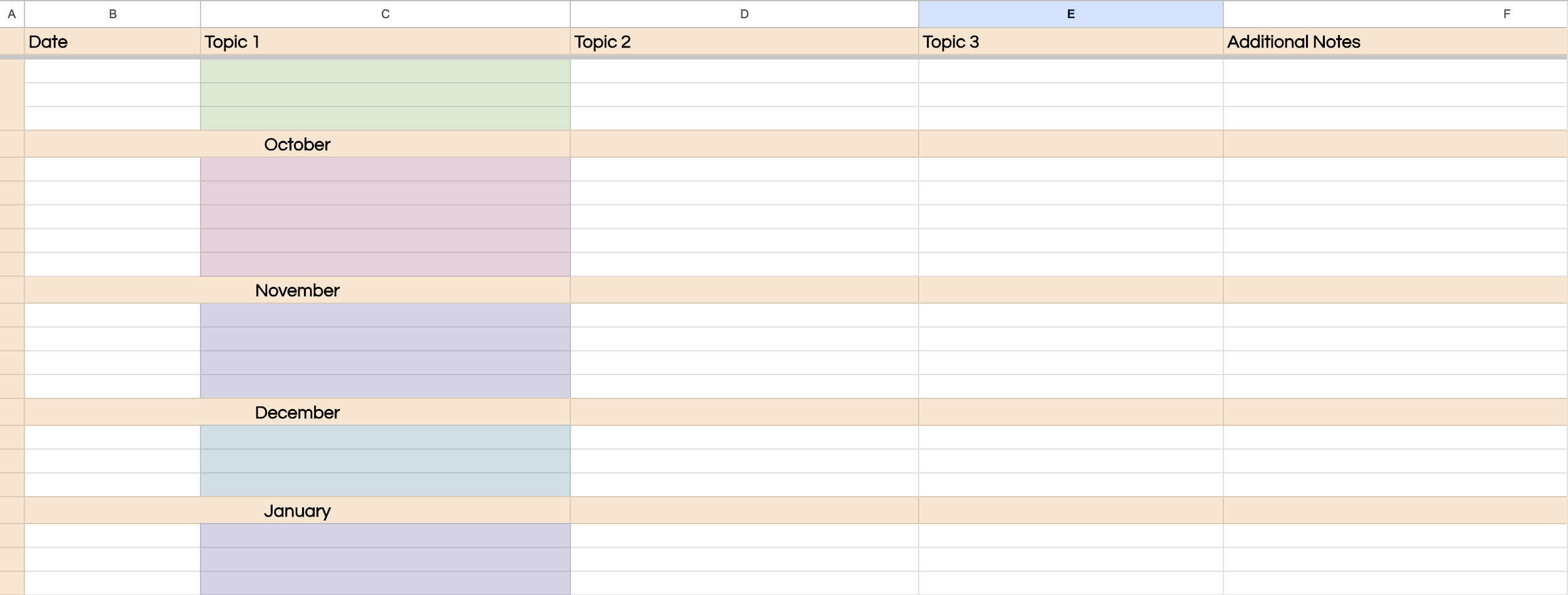

Sheets Setup
Ignoring any design from my screenshots - all credit goes to my much more creative wife - the setup for the sheet is fairly
simple. You need various headings in Row A of the sheet which we will be using to reference data. In this tutorial, our
headings are Date, Topic 1, Topic 2, Topic 3, Additional Notes. Whether you start on Row 1 or after that doesn’t matter too
much.
For the date column, we’ll be formatting our date like this: “February 26, 2024”. You’ll see why in a little bit.
On top of the actual data in the Sheet, the Apps Script is going to live in this document and just push data to the Slide. To
access your App Scripts, click Extensions > Apps Scripts. A new tab will open with a blank IDE style interface and an empty
myFunction.
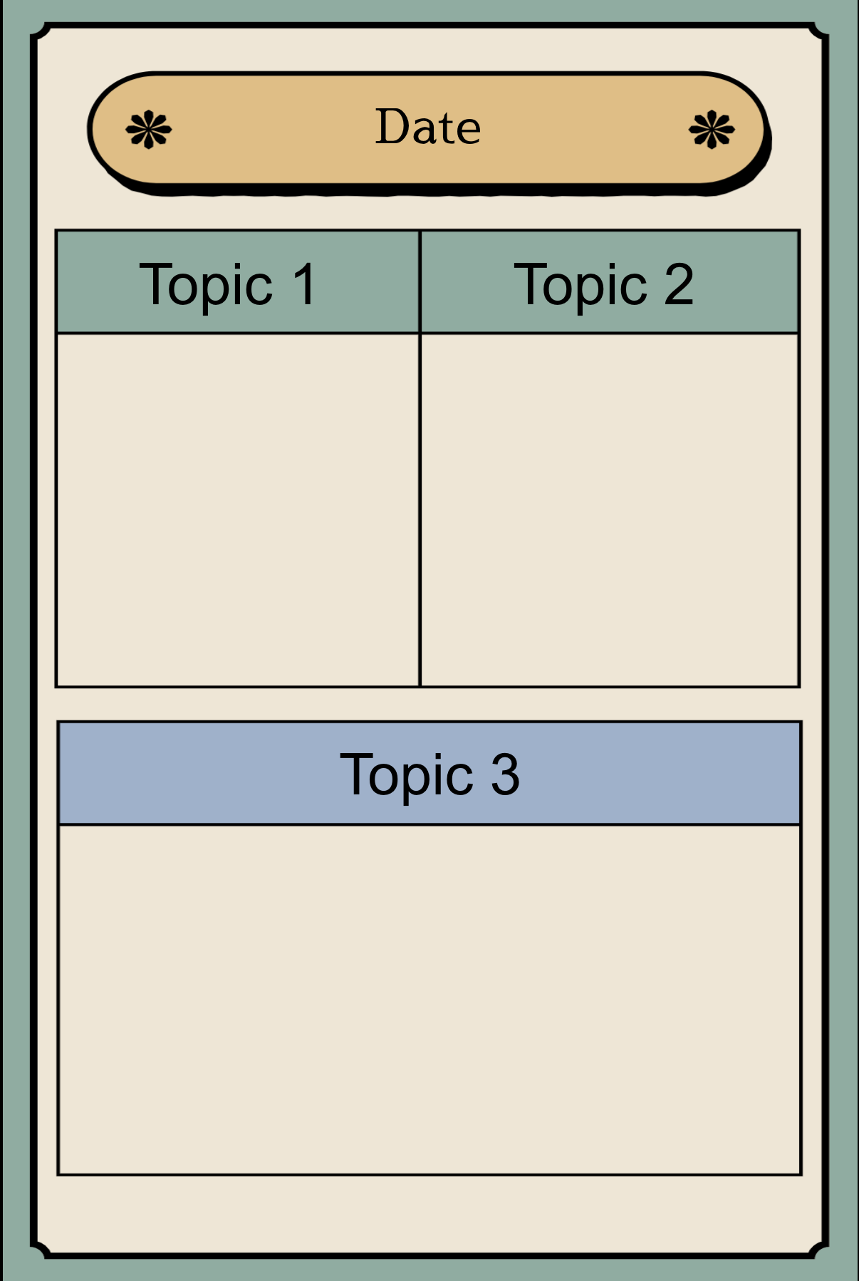
Slides Setup
Don’t worry too much about the design for Slides, you can change that later. But the important step is creating the empty text boxes. After you create your text boxes (4 will be used in this tutorial), right click one of them and select “Format Options”. A panel on the left hand-side should slide out. Click the “Alt Text” drop down, and then “Advanced Options”. That little text box is the title for your text box; it is not used in the visual representation of the box, we will just be using it as a reference point.
For ease of this tutorial, make the Title of the text box the same as the Header row from when we set up the Sheet, above. Once you’ve added title to each of the text boxes, let’s head into the code.
onOpen Function
The first function you need for creating a UI change in the Google Sheet is an onOpen function that will setup the UI when
the Sheet is open.
|
|
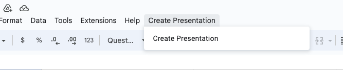
In this function (which we’ll later trigger in the script settings), when someone opens up the Sheet, it will create the UI button in the top level menu. Here’s what’s happening:
SpreadsheetApp.getUi()–> Instantiate class and get available methods forgetUi().createMenu()–> Creates a menu item called “Create Presentation”.addItem()–> Adds an item to that menu that when pressed, calls theaskDatefunction.addtoUi()–> Add it! Now people can see and click on it.
askDate Function
This is the main function and a bit long, so I’ll split it up into a few sections.
Section 1
|
|
This first section we’re just getting the sheet ready for analysis. With the dates variable, we’re just looking at the
second column. The reason we’re using the getDisplayValues() method is because Google will automatically convert the dates
to include time zone, time, etc. We want to keep the date in the same format for a better user experience.
For that last line, we’re getting the current date & time in epoch time so we can run a comparison further down the script. For this use case, we don’t need to include any dates in the past.
Section 2
|
|
In this section we’re creating an empty array and instantiating a RegExp to ensure we have an actual date in the cell. See Regex101 to learn more about Regex and test different regex syntax.
Something that threw me off when first writing this regex function was the way the Google IDE manages escape character and
slashes. If you take the second line above and input it into Regex101 you’ll see the \s or \d
become dark gray, basically skipping over that token. However, for Google, you’ll need an additional backslash to escape and
make the token become used by the function.
Here’s the “correct” RegExp string for Regex101.com: ^[A-Za-z]{3,15}\s\d{1,2},\s\d{2,4}
Next, we dive into a for loop, looping through the dates column of values (which we just called earlier). After attributing
each value to the var date variable, we also convert that same value into epoch time (by creating a new Date().getTime())
so that we can compare it with today’s date.
After the variables are setup we need to check that the date isn’t empty; we don’t need any rows where a date hasn’t been assigned to it yet. If we have a non-empty date value, let’s compare it using the regex string. All we’re doing here is asking “Is this date in the format I’m expecting it?” If true, let’s keep the value and continue using it. If not, just ignore it.
So we’ve now found a value that’s in the date format we expect, let’s now take that same value in epoch time (referenced by
the epochSheetDate variable) and compare it to today’s epoch time date. If today’s date is less than the value in the
sheet, that means the date in the sheet is in the future.
So now we have a date in the correct format and that is at some future date from today. Fantastic! Once we’ve gone through those checks, we’re ready to add the date to the array we created at the top of this section. Push on!
Section 3
|
|
This next section might feel long, but it’s really easy to follow, don’t worry. It’s a lot of data organization to ensure we’re giving the users a smooth experience & to make sure when the data hits the Slide, it’s in the right spot.
First things first - let’s only run this if we actually have items in the menuOptions array! No need to give the user an
affirmative message when there’s no data to process. If there are no dates available, we call the else of this if, which is
the 3rd to last line in this section.
A ui.alert is just a modal that offers no interaction to the user.
The next few lines are for processing that array of dates we grabbed from the sheet to making them presentable to the user.
Without the stringList and formattedDates variables, Google’s modal just shows a wall of text of dates which makes it
difficult to parse for the user. By using replaceAll() we remove the comma and insert a new line after every portion of the
string that contains 2024 and a comma.
So now, instead of the modal showing:
February 2, 2024,February 3, 2024,February 4,2024... etc
We now see the much easier to read:
February 2, 2024
February 3, 2024
February 4, 2024
After that’s formatted nicely, we can now have the prompt show for the user which asks them what date they would like to process into a Slide presentation. Since we haven’t visited any ui options since the top of this tutorial, this is the modal that will show up after a user clicks “Create Presentation” in the top level menu in Google Sheets.
Ok, so now moving onto line 5, we need to get the text for what the user enters into the modal box. If they don’t enter
anything, we should let them know that nothing will be done. That message comes from the second to last else statement in
this section. Instead, if they enter some data let’s parse it!
If you want to test yourself by adding in some new code try this exercise:
How can we ensure that the user entered a date in the format we expect? Tip: It is something reusable from another portion of the script.
For lines 9 and 10, we’re now looping back through the same set of rows that we did in section 2. The reason we’re re-entering this for loop is because we’ve already exited the loop. So we have to get the values again. Once we have them, let’s match the date that the user entered to the correct row. We’re able to do that by grabbing the index and adding 2 to it.
I haven’t fully looked into why we need to add 2 to get the correct row number. As we loop through the dates, the array
length (dates.length) is all the available rows in the sheet. So you would think that y is the row that the value is on;
but it’s not.
My only guess so far has to do with the frozen row at the top that I have in my Sheet. So the frozen row is not used, and row 2 is now index 0. Which means index 41 is technically row 43, and why we have to add 2 to the value to get the visually correct row number. We need this number to be correct so that we can get the rest of the values int he sheet.
Now that we have the correct row number, we’re going to shift from getting values from each row and getting them from each
column. By calling var presData = sheet.getRange(presRow,3,1,4).getValues(); we are grabbing an array. getRange is
looking for the following values, in the following order:
- Row number (which we got from the
y+2) - Column Number (which is Column C in this case)
- Number of Rows (we only need this row)
- Number of Columns (we know how many more columns we need).
Next up, we’re jumping into another for loop, now for all the data we just pulled from the column. This part is just parsing each column’s data into it’s own variable for easier management when we create the presentation. We’ve also grabbed the additional notes column, but we’re not using it right now. This column’s data may be valuable by adding it to the speaker notes of the Slide Presentation. Check out these two resources:
Once that’s done, call the next function: createPresentation()! We’re almost done.
createPresentation Function
|
|
This function may be the shortest to explain. All we are doing is taking those variables from the previous function (the variables that contain each topic’s text value) and doing the following:
- Opening the Presentation (line 2)
- Getting the first slide (line 3)
- Grabbing all the page elements (line 4)
- Looping through the page elements & grabbing all the titles that we set during setup (line 5 & 6)
- Then we compare the title of the Slide text box to the expected string (Topic 1-3), and if we get a match, retrieve the text of the box as a variable, clear the text, and input our new text with the variables we created in the previous function.
And just like that, you should have all your boxes filled in with the data you input to the Google Sheet!
Bonus exercises:
- Instead of overwriting this presentation each time, how can you add a new slide with the same text boxes? How would you find that slide since we’re right now grabbing the first slide?
- How can you change the name of this Slide Presentation to the date from the Sheet?
- Could you automatically export this Slide as a PDF and save it to a user’s Drive?
Full Script:
|
|